PINNs: When the Laws of Physics Guide Neural Networks
Table of contents7›
Over the past decade, the triumphant ascent of Deep Learning has rested almost exclusively upon an empirical cornerstone: extracting high-dimensional statistical patterns from titanic volumes of data. If the goal is detecting pedestrians on urban roadways, transcribing conversational audio in real time, or predicting the next token in a trillion-parameter frontier language model, the standard recipe remains unchanged: feed hundreds of thousands or millions of annotated examples into overparameterized neural networks, letting stochastic gradient descent adjust the synaptic weights.
Yet when artificial intelligence attempts to venture into the rigorous domains of theoretical physics, astrophysics, geophysics, or aerospace engineering, this empirical dogma collides head-on with physical reality: in the natural world, experimental data is inherently scarce, noisy, prohibitively expensive to acquire, or physically inaccessible. One cannot embed thousands of physical probes inside the hundred-million-degree plasma core of a magnetic confinement fusion tokamak, nor drill micro-sensors through the interior of a supersonic turbine blade in flight, nor measure the continuous 4D velocity vector field of blood flow through every microvascular capillary bed in the human brain.
Does it make sense to demand that a neural network learn the fundamental mechanics of the universe tabula rasa, forcing it to blindly rediscover from scratch the foundational conservation laws that humanity took three centuries to formalize? The answer to this epistemological question gave birth to one of the most vibrant and fertile paradigms in modern computational science: Scientific Machine Learning (SciML), and in particular, Physics-Informed Neural Networks (PINNs).
The Historical Genesis: From the Aegean Shores to the Laboratories of Brown
The fusion of classical continuum mechanics and deep learning did not emerge ex nihilo; rather, it crystallized through years of patient academic maturation led by researchers grounded in both rigorous numerical analysis and machine learning:
1. George Em Karniadakis and the Brown University School
The central figure in the modern realization of PINNs is Greek-American mathematician and engineer George Emmanouil Karniadakis (Γιώργος Εμμανουήλ Καρνιαδάκης; admired for his prolific unifying vision in forging an indissoluble epistemological bridge between continuum numerical analysis and deep neural networks; b. in Crete, Greece).
Born on the historic island of Crete in the southern Aegean Sea —a maritime cradle steeped in ancient seafaring and natural philosophy— Karniadakis displayed an early passion for fluid dynamics and continuum mechanics. He moved to Athens to study at the prestigious National Technical University of Athens (Ethnikó Metsóvio Polytechneío), earning his diploma in Mechanical Engineering and Naval Architecture in 1982.
 George Emmanouil Karniadakis, Charles Pitts Robinson and John Palmer Barstow Professor of Applied Mathematics at Brown University and Director of the CRUNCH research group. Source: Wikimedia Commons / CC BY-SA.
Eager to push the boundaries of scientific computing, he relocated to the United States to pursue graduate studies at the Massachusetts Institute of Technology (MIT), earning his Master of Science (Scientiae Magister, 1984) and his Ph.D. in Mechanical Engineering and Applied Mathematics in 1987 under the doctoral mentorship of Anthony T. Patera and Borivoje B. Mikić. His postdoctoral journey led him to the renowned Center for Turbulence Research at Stanford University and the NASA Ames Research Center, where he worked alongside turbulence modeling pioneers Parviz Moin and John Kim.
Following appointments as an assistant professor at Princeton University and visiting scholar at Caltech, Karniadakis joined the Division of Applied Mathematics at Brown University in Providence, Rhode Island, in 1994. There, he founded the influential CRUNCH research group and spearheaded the PhILMS consortium (Physics-Informed Learning Machines for Multiscale and Multiphysics Problems), sponsored by the United States Department of Energy (DOE). Globally celebrated for his pioneering contributions to spectral/hp-element methods for complex fluid geometries and uncertainty quantification in stochastic partial differential equations, Karniadakis realized early on that Deep Learning should not seek to replace mathematical physics, but rather serve as an organic, symbiotic partner.
2. The Hellenic Precursors: Isaac Lagaris and Trial Networks (1998)
While the contemporary PINN framework gained worldwide momentum between 2017 and 2019, its analytical blueprint was conceived two decades earlier. In September 1998, a team of Greek researchers at the University of Ioannina —led by Isaac E. Lagaris, Aristidis Likas, and Dimitrios I. Fotiadis— published a landmark paper in IEEE Transactions on Neural Networks entitled «Artificial neural networks for solving ordinary and partial differential equations».
Lagaris and his colleagues proposed formulating trial solutions wherein the output of a feedforward neural network was split into two analytical components: a predefined function strictly satisfying boundary or initial conditions, and a parameterized multilayer perceptron optimized to minimize the residual of the differential equation. In the late 1990s, however, computational hardware was severely constrained, classical sigmoid activations suffered from crippling vanishing gradients, and implementing differential operators required cumbersome symbolic derivations by hand for each specific problem.
3. The Modern Renaissance (2017–2019): Raissi, Perdikaris, and Karniadakis
In late 2017, two postdoctoral researchers in Karniadakis’s CRUNCH group at Brown, Maziar Raissi and Paris Perdikaris, authored two groundbreaking preprints that were published in 2019 in the Journal of Computational Physics: «Physics-informed neural networks: A deep learning framework for solving forward and inverse problems involving nonlinear partial differential equations».
The fundamental breakthrough achieved by Raissi, Perdikaris, and Karniadakis lay in harnessing modern reverse-mode Automatic Differentiation (AD) —a native engine of tensor computation frameworks like TensorFlow, PyTorch, and JAX. By leveraging AD, researchers were no longer bound to approximate spatial or temporal gradients with fragile finite-difference stencils, nor forced to derive unwieldy symbolic formulas: the neural network’s underlying computational graph itself calculates exact partial derivatives of the output with respect to continuous space and time coordinates.
The Mathematical Engine: How Does a PINN Learn?
To formalize how a PINN operates, consider a canonical nonlinear partial differential equation (PDE) parameterized across a continuous space-time domain $\Omega \times [0, T] \subset \mathbb{R}^d \times \mathbb{R}$:
$$\partial_t u(\mathbf{x}, t) + \mathcal{N}_{\mathbf{x}}[u(\mathbf{x}, t)] = 0, \quad \mathbf{x} \in \Omega, \quad t \in [0, T]$$
where $u(\mathbf{x}, t)$ denotes the physical state variable (such as velocity, pressure, or temperature) and $\mathcal{N}_{\mathbf{x}}$ represents a general nonlinear spatial differential operator (which may include advective convective terms $u \cdot \nabla u$ or dissipative terms $-\nu \Delta u$).
The dynamical system is completed by initial conditions at $t = 0$:
$$u(\mathbf{x}, 0) = g(\mathbf{x}), \quad \mathbf{x} \in \Omega$$
and boundary conditions on the spatial boundary $\partial\Omega$:
$$\mathcal{B}[u](\mathbf{x}, t) = h(\mathbf{x}, t), \quad \mathbf{x} \in \partial\Omega, \quad t \in [0, T]$$
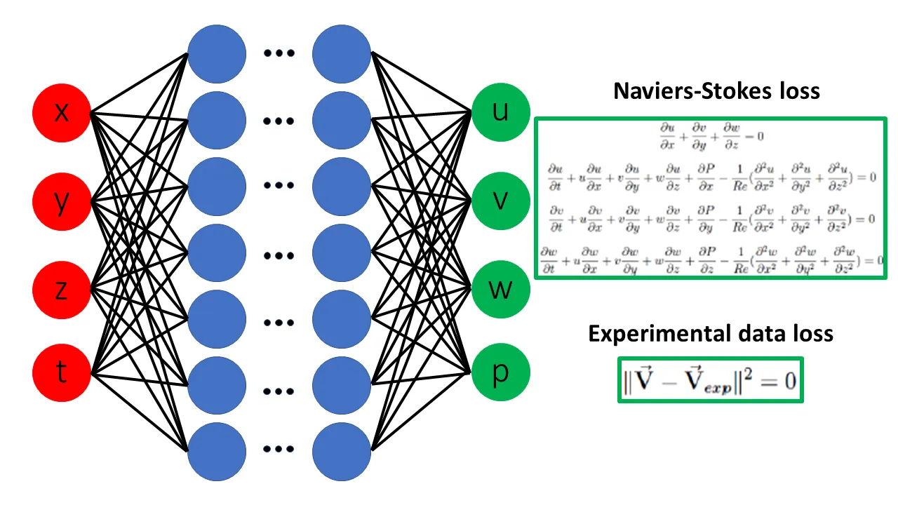 Computational architecture of a PINN: continuous space-time coordinates $(x, t)$ enter a multilayer perceptron generating output $\hat{u}$; automatic differentiation computes exact partial derivatives to evaluate the PDE residual, regularizing the composite loss function. Source: Wikimedia Commons / CC BY-SA 4.0.
1. Continuous Neural Field Approximation
Rather than discretizing the physical domain into an interconnected mesh of polyhedral cells as in traditional Finite Element Methods (FEM) or Finite Volume Methods (FVM), a PINN constructs a deep multilayer perceptron (MLP) parameterized by trainable weights and biases $\theta = {W^{(l)}, b^{(l)}}_{l=1}^L$:
$$\hat{u}(\mathbf{x}, t; \theta) = \sigma \left( W^{(L)} \dots \sigma(W^{(1)} [\mathbf{x}, t]^T + b^{(1)}) \dots + b^{(L)} \right)$$
where $\sigma(\cdot)$ is an infinitely differentiable activation function, such as the hyperbolic tangent ($\tanh$) or sinusoidal activations ($\text{Sin}$, popular in SIREN architectures).
2. The Physical Residual and Automatic Differentiation
The physical residual $r(\mathbf{x}, t; \theta)$ is evaluated by directly substituting the neural prediction $\hat{u}$ into the governing differential equation:
$$r(\mathbf{x}, t; \theta) := \partial_t \hat{u}(\mathbf{x}, t; \theta) + \mathcal{N}_{\mathbf{x}}[\hat{u}(\mathbf{x}, t; \theta)]$$
If $\hat{u}$ perfectly respects the physical conservation laws prescribed by the PDE, this residual vanishes identically across the continuum: $r(\mathbf{x}, t; \theta) \equiv 0$.
Here lies the mathematical brilliance of the method: partial derivatives such as $\frac{\partial \hat{u}}{\partial t}$, $\frac{\partial \hat{u}}{\partial x_i}$, and $\frac{\partial^2 \hat{u}}{\partial x_i \partial x_j}$ are not approximated via numerical finite-difference stencils (such as $\frac{\hat{u}(x+\Delta x) - \hat{u}(x)}{\Delta x}$), which introduce spatial truncation errors and struggle severely on irregular boundaries. Instead, the network’s directed acyclic computational graph systematically executes the multivariable chain rule backwards via reverse-mode automatic differentiation, computing partial derivatives with machine precision.
3. Mesh-Free Collocation Sampling
Evaluating the physics residual requires no rigid geometrical mesh. Instead, one samples an unstructured set of $N_f$ continuous collocation points scattered throughout the interior space-time domain:
$${(\mathbf{x}f^{(i)}, t_f^{(i)})}{i=1}^{N_f} \subset \Omega \times [0, T]$$
These points can be drawn using quasi-Monte Carlo techniques, such as Latin Hypercube Sampling (LHS) or low-discrepancy Sobol sequences, ensuring optimal spatial coverage without mesh-generation bottlenecks.
4. The Composite Multi-Objective Loss Function
Training a PINN amounts to solving a non-convex optimization problem where a composite loss function balances competing physical and observational demands:
$$\mathcal{L}(\theta) = w_{\text{data}} \mathcal{L}{\text{data}}(\theta) + w{\text{pde}} \mathcal{L}{\text{pde}}(\theta) + w{\text{bc}} \mathcal{L}{\text{bc}}(\theta) + w{\text{ic}} \mathcal{L}_{\text{ic}}(\theta)$$
where individual mean squared error (MSE) components are formulated as:
- PDE Residual Loss: $$\mathcal{L}{\text{pde}}(\theta) = \frac{1}{N_f} \sum{i=1}^{N_f} \left| r(\mathbf{x}_f^{(i)}, t_f^{(i)}; \theta) \right|^2$$
- Boundary Condition Loss: $$\mathcal{L}{\text{bc}}(\theta) = \frac{1}{N_b} \sum{i=1}^{N_b} \left| \mathcal{B}[\hat{u}](\mathbf{x}_b^{(i)}, t_b^{(i)}; \theta) - h(\mathbf{x}_b^{(i)}, t_b^{(i)}) \right|^2$$
- Initial Condition Loss: $$\mathcal{L}{\text{ic}}(\theta) = \frac{1}{N_0} \sum{i=1}^{N_0} \left| \hat{u}(\mathbf{x}_0^{(i)}, 0; \theta) - g(\mathbf{x}_0^{(i)}) \right|^2$$
- Observational Data Loss (from sparse sensors): $$\mathcal{L}{\text{data}}(\theta) = \frac{1}{N_d} \sum{i=1}^{N_d} \left| \hat{u}(\mathbf{x}d^{(i)}, t_d^{(i)}; \theta) - u{\text{sensor}}^{(i)} \right|^2$$
Weighting parameters $w_{\text{data}}, w_{\text{pde}}, w_{\text{bc}}, w_{\text{ic}}$ dynamically regulate gradient balance across objectives during optimization.
The Fundamental Duality: Forward vs. Inverse Problems
The PINN paradigm manifests a remarkable mathematical symmetry when addressing two classical scientific tasks:
1. Forward Problems (Direct Simulation)
In a forward problem, all physical parameters and material constants (e.g., kinematic viscosity $\nu = 0.01$, fluid density $\rho = 1.0$) are known, alongside initial and boundary conditions. The neural network operates as a continuous mesh-free numerical integrator. Using first-order optimizers (Adam) followed by second-order quasi-Newton algorithms (L-BFGS), the network converges toward the continuous solution field without generating millions of geometrical elements.
2. Inverse Problems (System Identification & Physics Discovery)
The inverse problem represents the true crown jewel of Scientific Machine Learning. In experimental science and industrial diagnostics, the structural form of the governing equations is often known, yet crucial material properties remain undetermined (such as the thermal conductivity of a novel superalloy, hydraulic permeability in subsurface aquifers, or wall elasticity in human coronary arteries).
In a PINN, unknown physical parameters $\boldsymbol{\lambda} = {\lambda_1, \lambda_2, \dots}$ are embedded directly into the computational graph as trainable latent variables alongside network weights $\theta$. Given sparse, noisy telemetry from a handful of physical sensors, the backpropagation algorithm simultaneously reconstructs the full continuous field across unmeasured regions (physics-based super-resolution) while pinpointing the exact numerical value of the unknown constitutive constants.
Frontier Applications: From Cardiovascular Hemodynamics to Additive Manufacturing
The adaptability of physics-informed learning has driven breakthroughs across multiple technical domains:
- Cardiovascular Hemodynamics and Precision Medicine:
Simulating pulsatile blood flow in patient-specific cerebral aneurysms and aortic dissections. By fusing sparse 4D Flow MRI scans with the incompressible Navier–Stokes equations, PINNs reconstruct near-wall velocity profiles and infer endothelial wall shear stress (WSS), an invaluable clinical biomarker for predicting aneurysm rupture. - Laser Additive Manufacturing (3D Printing):
Capturing ultra-fast phase transitions and thermal gradients in laser powder bed fusion processes. Incorporating nonlinear heat conduction and Stefan phase-change dynamics enables accurate prediction of residual thermal stresses, microstructural porosity, and structural fatigue in aerospace-grade titanium components. - Subsurface Hydrology and Carbon Sequestration:
Modeling multi-phase fluid flow in heterogeneous porous rock formations governed by Darcy–Brinkman equations, optimizing underground supercritical carbon dioxide ($CO_2$) storage and geothermal reservoir management. - Industrial Digital Twins:
Deploying lightweight neural surrogate models that execute in microseconds on edge devices or cloud microservices. Assimilating continuous real-time sensor streams from wind turbine farms or nuclear heat exchangers enables predictive maintenance and real-time operational safety assessments.
Open Theoretical Challenges and Epistemic Limits
Objective scientific communication requires acknowledging that PINNs are neither an effortless silver bullet nor free from significant theoretical hurdles:
- Gradient Pathologies:
The multi-objective loss landscape is fiercely non-convex. Groundbreaking studies by Sifan Wang and Paris Perdikaris (2021) demonstrated that gradient magnitudes from boundary loss components often differ by several orders of magnitude compared to PDE residual gradients. This imbalance causes standard optimizers to collapse into pathological local minima, where the network memorizes boundary values while failing to satisfy the governing physics in the interior. - Spectral Bias:
Standard neural networks suffer from an intrinsic spectral bias: they preferentially learn low-frequency spatial patterns rapidly, requiring thousands of additional training iterations to resolve localized shock waves, boundary layers, or fine-scale turbulence. - Temporal Causality Breakdown:
In transient time-dependent PDEs, optimizing simultaneously across the full space-time cylinder $\Omega \times [0, T]$ violates physical causality: the optimizer attempts to satisfy the physics at late times ($t = T$) before properly resolving dynamics at early times ($t \to 0$), often leading to catastrophic simulation failures. - Computational Cost vs. Classical Solvers:
For forward simulations on standard geometries where well-refined meshes already exist, mature finite element (FEM) or finite volume (FVM) solvers (such as OpenFOAM, ANSYS, or FEniCS) remain significantly faster and orders of magnitude more computationally efficient than training a deep PINN from scratch. The true competitive advantage of PINNs emerges in inverse problems, high-dimensional parameter spaces, multi-modal sensor fusion, or geometrically intricate scenarios where conventional mesh generation fails.
To transcend these constraints, cutting-edge research is rapidly evolving toward Neural Operator Learning, notably DeepONet —conceived by Karniadakis’s team— and Fourier Neural Operators (FNO), designed to learn continuous nonlinear mappings directly between infinite-dimensional function spaces.
Reflection: The Dialogue Between Data and Universal Law
The classical Greek term physis (φύσις) originally denoted the intrinsic, self-organizing order of the cosmos—the generative principle and the silent, immutable laws that govern the motion of all things.
For years, the intoxicating power of modern Big Data fostered the reductionist illusion that classical analytical laws —conceived by towering minds like Newton, Euler, Fourier, Navier, and Stokes— could be rendered obsolete by blind, data-hungry algorithms. The emergence of Physics-Informed Neural Networks serenely dispels that hubris: it reminds us that computational intelligence achieves its purest elegance not by casting aside fundamental first principles, but by standing upon their shoulders and letting mathematical truth illuminate the path forward.
References and Verified Sources
- Raissi, M., Perdikaris, P., & Karniadakis, G. E. (2019): Physics-informed neural networks: A deep learning framework for solving forward and inverse problems involving nonlinear partial differential equations. Journal of Computational Physics, vol. 378, pp. 686–707. DOI: 10.1016/j.jcp.2018.10.045 | Preprint on arXiv:1711.10561.
- Raissi, M., Perdikaris, P., & Karniadakis, G. E. (2017): Physics Informed Deep Learning (Part II): Two-dimensional Navier-Stokes, Euler and Klein-Gordon Equations. arXiv:1711.10566.
- Lagaris, I. E., Likas, A., & Fotiadis, D. I. (1998): Artificial neural networks for solving ordinary and partial differential equations. IEEE Transactions on Neural Networks, vol. 9, no. 5, pp. 987–1000. DOI: 10.1109/72.712178.
- Karniadakis, G. E., Kevrekidis, I. G., Lu, L., Perdikaris, P., Wang, S., & Yang, L. (2021): Physics-informed machine learning. Nature Reviews Physics, vol. 3, no. 6, pp. 422–440. Nature Reviews Physics.
- Lu, L., Jin, P., Pang, G., Zhang, Z., & Karniadakis, G. E. (2021): Learning nonlinear operators via DeepONet based on the universal approximation theorem of operators. Nature Machine Intelligence, vol. 3, no. 3, pp. 218–229. arXiv:1907.04502.
- Wang, S., Teng, Y., & Perdikaris, P. (2021): Understanding and mitigating gradient pathologies in physics-informed neural networks. SIAM Journal on Scientific Computing, vol. 43, no. 5, pp. A3055–A3081. arXiv:2001.04385.
- Brown University CRUNCH Group: Scientific Machine Learning & Multiscale Modeling. Official research lab portal led by George Karniadakis. CRUNCH Group at Brown.